Three-dimensional (3D) obstacles on the bottom are common sites for the generation of vortices, internal waves and turbulence by ocean currents. Turbulence-resolving simulations are conducted for stratified flow past a conical hill, a canonical example of 3D obstacles. Motivated by the use of slip boundary condition (BC) and drag-law (effectively partial slip) BC in the literature on geophysical wakes, we examine the sensitivity of the flow to BCs on the obstacle surface and the flat bottom. Four BC types are examined for a non-rotating wake created by a steady current impinging on a conical obstacle, with a detailed comparison being performed between two cases, namely NOSL (no-slip BC used at all solid boundaries) and SL (slip BC used at all solid boundaries). The other two cases are as follows: Hybrid, undertaken with slip at the flat bottom and no-slip at the obstacle boundaries, and case DL wherein a quadratic drag-law BC is adopted on all solid boundaries. The no-slip BC allows the formation of a boundary layer which separates and sheds vorticity into the wake. Significant changes occur in the structure of the lee vortices and wake when the BC is changed. For instance, bottom wall friction in the no-slip case suppresses unsteadiness of flow separation leading to a steady attached lee vortex. In contrast, when the bottom wall has a slip BC (the SL and Hybrid cases) or has partial slip (DL case), unsteady separation leads to a vortex street in the near wake and the enhancement of turbulence. The recirculation region is shorter and the wake recovery is substantially faster in the case of slip or partial-slip BC. In the lee of the obstacle, turbulent kinetic energy (TKE) for case NOSL is concentrated in a shear layer between the recirculating wake and the free stream, while TKE is bottom-intensified in the other three cases. DL is the appropriate BC for high-𝑅𝑒 wakes where the boundary layer cannot be resolved. The sources of lee vorticity are also examined in this study for each choice of BC. The sloping sides lead to horizontal gradients of density at the obstacle, which create vorticity through baroclinic torque. Independent of the type of BC, the baroclinic torque dominates. Vortex stretch and tilt are also substantial. An additional unstratified free-slip case (SL-UN) is simulated and the wake is found to be thin without large wake vortices. Thus, stratification is necessary for the formation of coherent lee vortices of the type seen in geophysical wakes.

Streamlines

Instantaneous streamlines which originate from upstream are plotted at 𝑡∗ = 100: (a) NOSL and (b) SL. The streamlines are colored with the vertical velocity. The silver blue color represents the isosurface 𝑢 = 0, which demarcates the recirculation zone behind the obstacle up to 𝑥∗ = 2.2 downstream.

Mean Streamwise Velocity

Mean streamwise velocity (a–b) and vertical velocity (c–d) in the horizontal plane 𝑧∗ = 0.5. Aspect ratio of figure axes is 1:1. The dotted white line denotes the 𝑢 = 0 contour.

Lee Vortices

The organization of the lee vortices is affected by the boundary conditions. Lee vortices are shown by contours of normalized vertical vorticity at 𝑡∗ = 100: (a) NOSL, and (b) SL.

Density

Streamwise and lateral gradients in density, visible from contours of the density deviation (𝜌∗) from the background, in the horizontal plane 𝑧∗ = 0.5: (a) NOSL, and (b)SL.

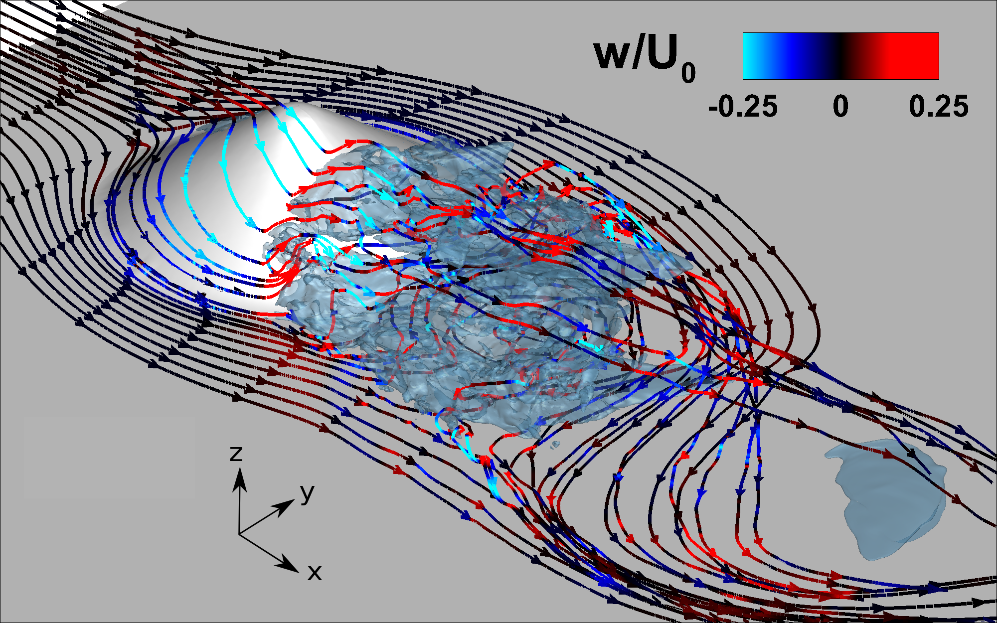
The effect of ambient stratification on flow past a prolate spheroid is investigated using large-eddy simulation. The aspect ratio of the body is L/D = 4 and the major axis (L) is aligned with the incoming flow. The Reynolds number based on the minor axis (D) and the incoming velocity (U) is Re = 104. The stratification is set using a linear density background with constant buoyancy frequency (N). Three simulations with stratification levels, Fr = U/ND = 0.5, 1, 3 and one unstratified simulation, Fr=∞, are performed. The influence of the body slenderness ratio is assessed by comparing the present results with previous work on a sphere. An overall result is that the flow past a slender body exhibits stronger buoyancy effects relative to a bluff body. At Fr ∼ O(1), there is a strong interaction between the body-generated internal gravity waves (IGW) and the flow at the body. This interaction gives rise to a critical Froude number, Frc = L/Dπ, which is proportional to the aspect ratio. When Fr ≈ Frc boundary layer separation is delayed and wake turbulence is strongly suppressed. If Fr >≈ Frc, wake turbulence is only partially suppressed and, when Fr <≈ Frc, boundary layer separation is promoted and turbulence reappears. To elucidate the effect of body slenderness on stratification effects, the IGW field, the boundary layer evolution and separation are studied. Analysis of the wake reveals the strong influence of the type of separation, and therefore the body shape, on the dimensions and the energetics of the near and intermediate wake. However, the decay rate of the stratified wake in the nonequilibrium region is the same as that of a sphere.

Internal Gravity Waves

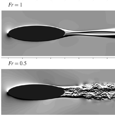
Internal gravity waves, visualized by contours of vertical velocity (w): (a) Fr = 0.5, (b) Fr = 1, (c) a zoom of Fr = 1 to highlight the inclined phase lines on the body, and (d) Fr = 3. The black solid lines in each panel represent the w = 0 phase lines obtained with the asymptotic theory for the far field. The gray dashed lines in each panel mark the phase lines of w = 0 obtained by the near-field theory.

Streamlines

Effect of Fr on the streamlines starting from the nose of the body. The streamlines are colored by vertical velocity. The blue isosurface in the aft of the body marks the points where the streamwise velocity u = 0.

Boundary Layer

Effect of Fr on the BL velocity profiles along the vertical (top row) and horizontal (bottom row) planes. The velocity is shown as a function of the nondimensional normal distance to the wall, n. Different streamwise locations are shown: left column corresponds to x = −1, middle column to x = 0, and right column to x = 1.

Wake

Effect of stratification on the streamwise evolution of overall wake properties: (a) half-height (LV ), (b) half-width (LH ), (c) center line defect velocity (Ud ), and (d) turbulent kinetic energy (TKE).

Since first discovered many decades ago in the Pacific Equatorial Undercurrents (EUC), processes leading to deep-cycle (DC) turbulence remain a mystery. The night-time DC turbulence causes enhanced mixing in the marginally-unstable regions where background shear and stratification are strong due to the presence of the EUC and the thermocline. Numerous mechanisms leading to DC turbulence have been proposed such as obstacle effects, local shear instability, breaking internal waves, etc.; however, further evidence is needed in order to support the proposed mechanisms. Understanding the processes leading to the DC turbulence and its associated mixing is of practical interest because it plays a crucial role in the heat budget of upper equatorial oceans, and therefore, can affect global climate.

We constructed LES simulations based on the observational data to quantify the amount of mixing by the DC turbulence. Some important findings that I discover are: (1) a new mechanism that can trigger the DC turbulence via marginal instability (Pham et al. 2012, Pham et al. 2013, Smyth et al. 2017}; and (2) an explanation of why the observed DC turbulence in the spring is significantly weaker than in other seasons (Pham et al. 2017}. Recently, we begin to investigate the effect of marginal instability and DC turbulence on the warming of SST during the 2014-2016 El Niño Southern Oscillations (ENSO) event.

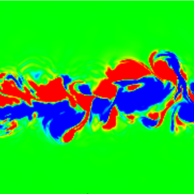
Figure 1 contrasts sea surface temperature (SST) during the weak 2014 El Niño (upper) and the strong 2015 El Niño (lower). The event caused a record high SST anomaly as the cold tongue withdrew toward the Central American coast. We will use a combination of observational data, DNS and LES to quantify and parametrize turbulent mixing during this time period. A preliminary result is shown in Figure 2. Here, we performed DNS of a stratified shear flow at a high Reynolds number to explore how the evolution of shear instabilities controls the rate of turbulent mixing. DNS provides an accurate quantification of the rate of mixing which can be used to assess mixing parameterization schemes used in general circulation models.

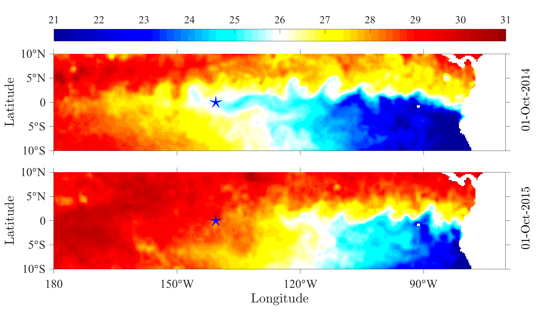
Figure 1: Warming of sea surface temperature (SST) across the Pacific Ocean during the record-high 2014-2016 ENSO. It is of interest to explore how turbulent mixing contributes to the warming of SST during this period using LES and DNS. Remote sensing data are taken from the Group for High Resolution Sea Surface Temperature (GHRSST).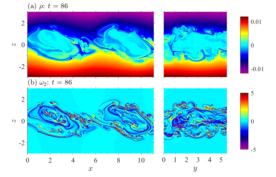

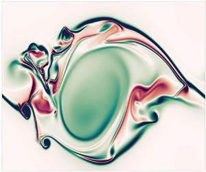
Figure 2: Route to mixing in the DNS of a stratified shear layer at a high Reynolds number. The mixing is driven by the primary Kelvin-Helmholtz shear instabilities and a myriad of secondary instabilities.

The objective of the present study, based on four phases, is to employ DNS and LES to further understand and quantify the dynamical processes underlying turbulenceduring the generation of an internal wave beam and its subsequent interaction with arealistically-stratified upper ocean. In the first phase, a study of a stratified non-sloping bottom boundary layer under an oscillating tide has been completed and published by Gayen et al. JFM (2010). Here, we observed that stratification decreases phase lag with respect to free stream velocity for various boundary layer properties over the course of the cycle. Turbulence generated internal waves are observed to propagate external to boundary layer. Phase angle of IW changes over tidal cycle. The frequency spectrum of the propagating wave is found to span a narrow band of frequencies corresponding to clustering around 45^o.

In second phase, three-dimensional DNS has been performed of generation by a laboratory-scale slope in the regime of excursion number, Ex ≪ 1, and criticality, e ≃ 1, that shows transition to turbulence. The transition is found to be initiated by a convective instability which is closely followed by shear instability. Turbulence is present along the entire extent of the near-critical region of the slope. The wave energy exhibits a temporal cascade to higher harmonics, subharmonics and inter harmonics. Recently, this work has been published in Gayen & Sarkar, Phys. Rev. Lett.(2010). The work of Gayen & Sarkar, JFM (2011) extends the previous work by examining internal wave energetics as well as the energetics of turbulence in the bottom boundary layer.The peak value of the near-bottom velocity is found to increase with increasing length of the critical region of the topography. The scaling law that is observed to link the near-bottom peak velocity to slope length is explained by an analytical boundary layer solution that incorporates an empirically obtained turbulent viscosity. The slope length is also found to have a strong impact on quantities such as the wave energy flux, turbulent production and turbulent dissipation. These sets of numerical experiments that explain and characterize turbulence during the generation of internal waves from tide-topography interaction at near-critical environment constitute the second phase of work.

Our main goal in the third phase is to scale up the computational domain which has been used in second phase, from O(10)m to O(1) km in order to reproduce the large scale overturns observed in the ocean and compare the wave energetics, turbulent statistics etc. with the available measured data. Here, we have taken a beam of 60 m width and amplitude of 0.125 m/s to study the mixing dynamics over a sloping topography under near critical environment. Large value of tke as well as large values of of positive buoyancy flux at elevated level is observed during the flow reversal from downslope to upslope motion (Ref. Gayen & Sarkar, Geophys. Res. Lett. (2011))

The objective of the forth phase is to understand the interaction process between internal tidal beam and realistic upper ocean stratification and to characterize the role turbulence.

Phase I: Turbulence and internal waves at non-sloping bottom under an oscillating tide

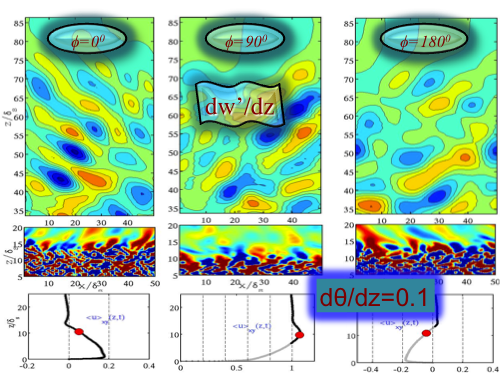
Slice of ∂w/∂z in the x–z plane for the case with Ri=500 at different tidal phases: (a) φ =−5◦, (b) φ =90◦ and (c) φ =180◦. Each part is divided into three panels: top panel shows the waves in the far-field, z=35−86; middle panel shows the turbulent source and near-field waves; bottom panel shows the streamwise velocity profile with black and light grey indicating positive and negative signs of the velocity relative to the free steam. The O symbols on the velocity profiles show the location of ∂θ(z, t )/∂z=0.1 to demarcate the mixed layer.

Phase II: Turbulence and internal waves at sloping bottom under an oscillating tide

Internal wave field visualized by a slice of dw/dz field in x-z plane.

Phase III: Boundary mixing by density overturns in an internal tidal beam

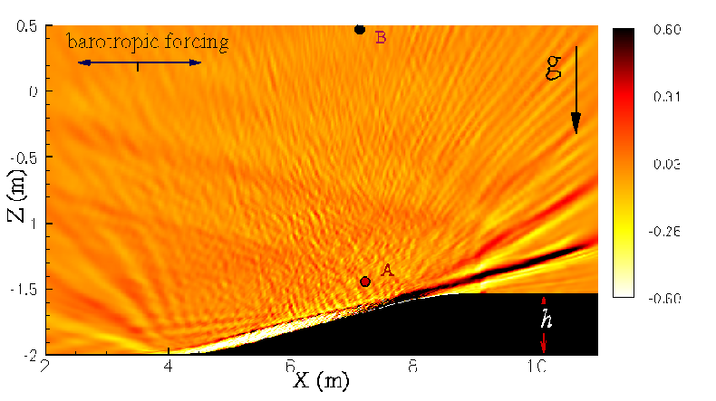
Bottom panel shows vertical x-z slice of the density field (after subtracting 1000 kg m −3) at 4 different times (phases) in a tidal cycle. Top panel shows spanwise-averaged streamwise velocities, u(z, t) m/s and density profiles, ρ(z, t, x = 0) at corresponding phases. Background linear density (dashed blue line) profile is also shown. Note that u, x are horizontal while z is vertical. Parts (a) and (e) correspond to maximum downward boundary flow, parts (b) and (f) correspond to flow reversal from down to up, parts (c) and (g) correspond to peak up-slope velocity and, finally, parts (d) and (e) correspond to flow reversal from up to down. The four different times are indicated by the four red color circles in Figure 4a that follows. Here, arrows are pointing the ow structures.

Phase IV: Interaction of IW beam with pycnocline and turbulence

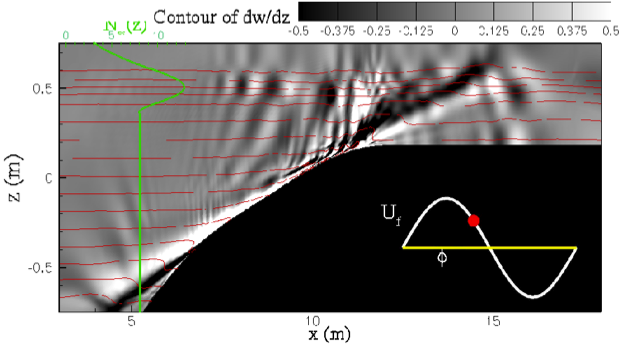
Preliminary results show an upward wave beam incident on realistic upper ocean stratification (buoyancy frequency profile is the green curve on the left). The phase of the barotropic tidal currents (white sine curve) is shown by the red dot. This figure is taken from ongoing work performed by Gayen and Sarkar.

While the turbulent wake behind a moving body is a fundamental problem in turbulence and has been studied for hundreds of years, even the wake behind relatively simple shapes such as spheres still lacks a complete description. The reason for this is that the wake is highy nonlinear which makes it difficult to study analytically. The presence of a density gradient significantly complicates matters as it destroys the symmetry of the problem and introduces a complex coupling between kinetic and potential energy.

For studying the wake behind a bluff body there are two configurations that are commonly used: a towed body and a self-propelled body. The wake profiles for the two configurations are qualitatively different. The wake of a towed body consists solely of a drag lobe whereas the wake of a self-propelled body consists of both a drag lobel and a thrust lobe. For a self-propelled body moving at constant speed, the drag and thrust balance which produces a wake with zero net momentum. If a self-propelled body is accelerating then it will have a wake with excess momentum. The presence of a density gradient disrupts the balance of momentum in the wake of a self-propelled body moving at constant speed by inhibiting motion in the vertical direction and allowing the presence of internal gravity waves which carry energy away from the wake to the surroundings.

All stratified turbulent wakes follow a qualitatively similar evolution. First there is a near wake region where the wake evolves as thought it was unstratified. The next region is termed the Non-Equilibrium regime where the wake feels the effect of buoyancy. During this time the wake slowly collapses in the vertical direction and expands in the horizontal direction. The collapse generates internal gravity waves which propagate energy from the wake to the background. At late time, the Q2D regime, the flow is quasi-horizontal and decays until the wake relaminarizes. Large pancake eddies form in the Q2D regime.

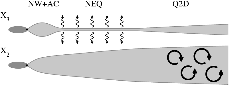
Wake evolution in the vertical, x3, and horizontal, x2, directions. Wavy arrows show the time when wake generated internal gravity waves are significant and pancake eddies are shown in the late wake.

The mean velocity in the wake behind a body moving to the left. (a) Towed body. (b) Self-propelled body with zero net momentum. (c) propelled body with excess momentum.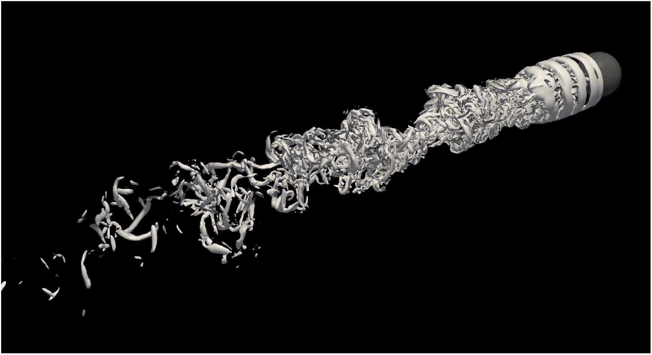

Unstratified flow past a sphere at Re = 3700. Picture shows isosurface of vortical structure captured by Q-criterion at Q = 1. Vortical structures appear to be tube-like, so called "vortex tube".

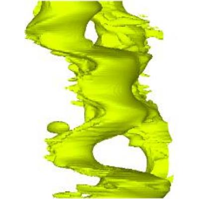
Isolated horizontal shear is a feature of boundary currents, flow near river deltas, and wakes of topographical features. The picture below shows a shear layer resulting from separation of a boundary current. Mixing and transport induced by vertical shear in a stably stratified fluid has been explored far more extensively than that case of horizontal shear. We are interested in the effects of stratification strength and rotation rate on flow dynamics. When stratification is strong, vertical gradients can dominate the flow and new instability mechanisms such as the zigzag instability emerge. The zigzag instability is shown below along with a vortex taken from a simulation of a stratified horizontal shear layer. The effects of rotation are non-negligible when length scales are of order 1 kilometer. Rotation can either stabilize or destabilize a flow field, depending on rotation rate and orientation.

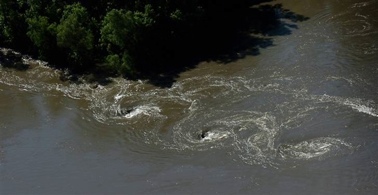
Horizontal shear layer in a river.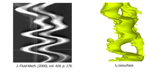

Zigzag instability. (left image) Experiment. (right image) Simulation.

The project is focused, via numerical experiments, on the conversion of barotropic tides into internal tides and the effect of turbulence generated near the topography on the conversion. The Navier-Stokes equations are solved using a mixed RK3-ADI time integration scheme. Immersed Boundary Method module is developed to include the effect of three dimensional rough topography on a cartesian grid. At the initial phase of the project, direct and large eddy simulations are performed to study tidal flow over a model ridge. The Navier-Stokes equations are solved in generalized coordinates using a mixed spectral-finite difference algorithm. The effect of criticality parameter on the tidal conversion is studied in the laminar flow regime. Nonlinear processes become important at critical slope of the topography even for low excursion numbers. The effect of turbulence on tidal conversion is studied under near-critical flow conditions. Physical quantities of interest include the kinetic energy, power spectra, vertical turbulence intensity and buoyancy flux.

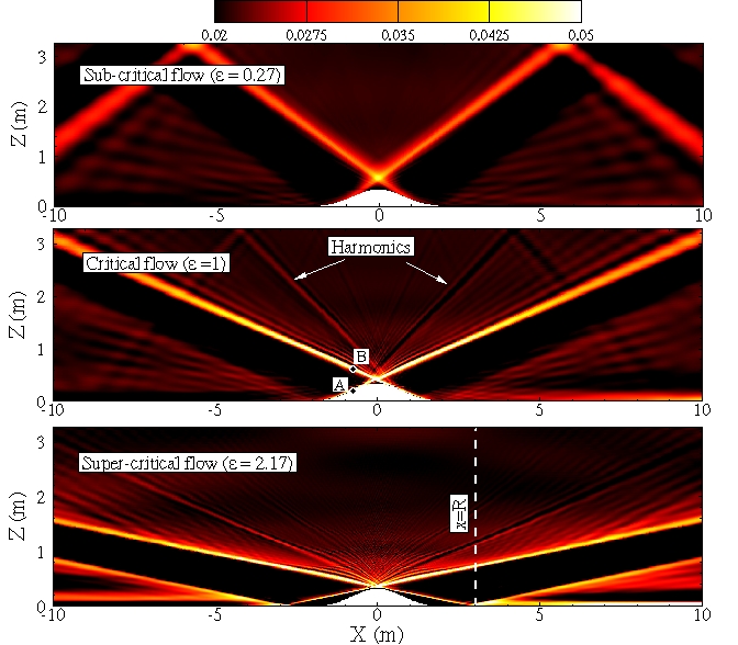
Comparison between the subcritical, critical and supercritical flows at Res=30.

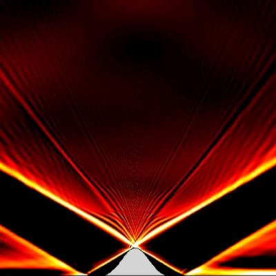
urms near the topography for critical flow at Res=30.

Direct numerical simulation is performed to study the internal gravity wave reflection on a sloping boundary, considering near critical slope angles. Our objective is to understand the role of near critical slopes in mixing near the boundaries during internal wave reflection. The wave field includes only the reflected wave, this is done by imposing velocity and density boundary conditions for the reflected wave at the sloping bottom. Two different scenarios have been considered, first by keeping slope angle constant and studying the effect of Froude number, second by keeping Froude number constant and varying the slope angle. With increasing Froude number, the reflection process becomes increasingly nonlinear with the formation of higher harmonics and subsequently fine scale turbulence. At a critical value of Froude number, turbulence is initiated via convective instability. Also, turbulent intensities are more pronounced for somewhat off-critical reflection compared to exactly critical reflection. As the Froude number increases, the near wall shear plays a dominant role in critical reflection by enhancing turbulence compared to off-critical reflection. For a fixed slope angle, as the Froude number increases the fraction of the input energy converted into the turbulent kinetic energy increases and saturates at higher Froude numbers.

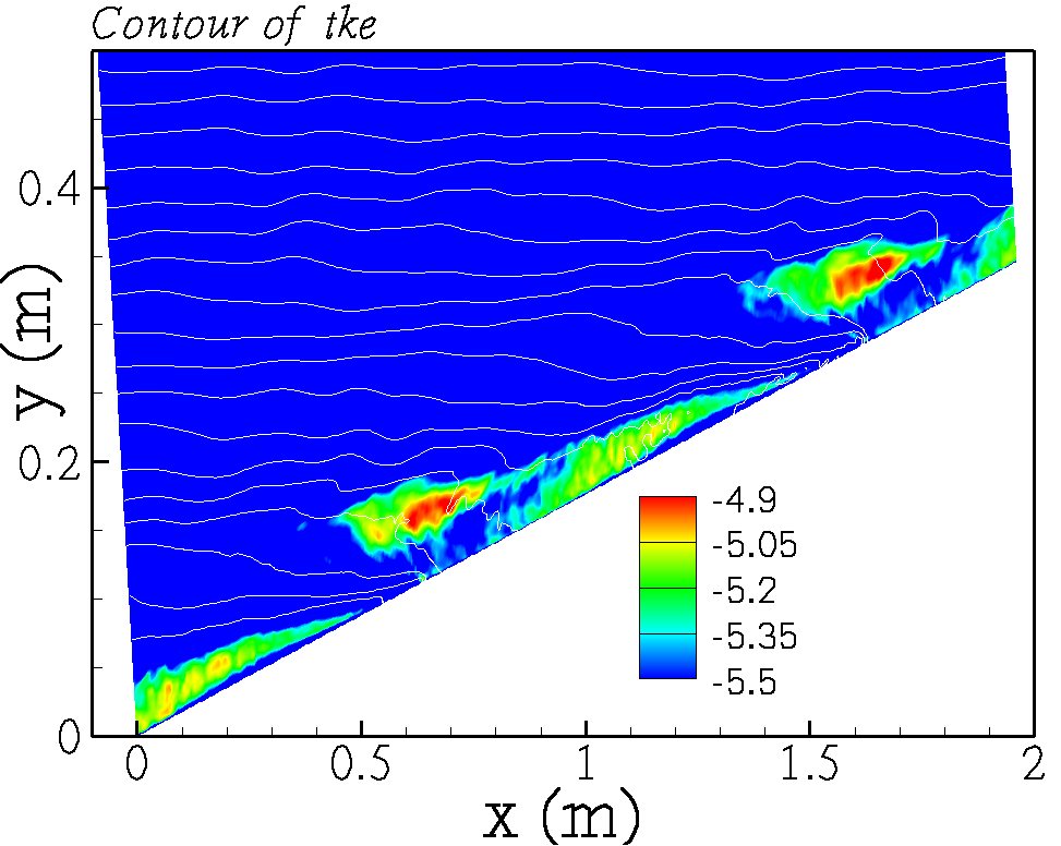
Contour of turbulent kinetic energy.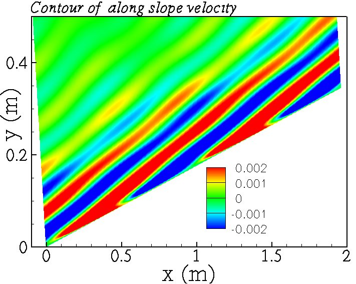

Contour of along slope velocity.