Computational Fluid Dynamics Laboratory

Internal wave field during a tidal flow over a sloping topography

My interest is in the broad area of Geophysical Fluid Dynamics which focuses on turbulence and internal waves in tidal flow over topography via numerical experiments.

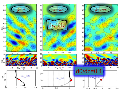
The objective of the present study, based on four phases, is to employ DNS and LES to further understand and quantify the dynamical processes underlying turbulenceduring the generation of an internal wave beam and its subsequent interaction with arealistically-stratified upper ocean. In the first phase, a study of a stratified non-sloping bottom boundary layer under an oscillating tide has been completed and published by Gayen et al. JFM (2010). Here, we observed that stratification decreases phase lag with respect to free stream velocity for various boundary layer properties over the course of the cycle. Turbulence generated internal waves are observed to propagate external to boundary layer. Phase angle of IW changes over tidal cycle. The frequency spectrum of the propagating wave is found to span a narrow band of frequencies corresponding to clustering around 45^o.

In second phase, three-dimensional DNS has been performed of generation by a laboratory-scale slope in the regime of excursion number, Ex ≪ 1, and criticality, e ≃ 1, that shows transition to turbulence. The transition is found to be initiated by a convective instability which is closely followed by shear instability. Turbulence is present along the entire extent of the near-critical region of the slope. The wave energy exhibits a temporal cascade to higher harmonics, subharmonics and inter harmonics. Recently, this work has been published in Gayen & Sarkar, Phys. Rev. Lett.(2010). The work of Gayen & Sarkar, JFM (2011) extends the previous work by examining internal wave energetics as well as the energetics of turbulence in the bottom boundary layer.The peak value of the near-bottom velocity is found to increase with increasing length of the critical region of the topography. The scaling law that is observed to link the near-bottom peak velocity to slope length is explained by an analytical boundary layer solution that incorporates an empirically obtained turbulent viscosity. The slope length is also found to have a strong impact on quantities such as the wave energy flux, turbulent production and turbulent dissipation. These sets of numerical experiments that explain and characterize turbulence during the generation of internal waves from tide-topography interaction at near-critical environment constitute the second phase of work.

Our main goal in the third phase is to scale up the computational domain which has been used in second phase, from O(10)m to O(1) km in order to reproduce the large scale overturns observed in the ocean and compare the wave energetics, turbulent statistics etc. with the available measured data. Here, we have taken a beam of 60 m width and amplitude of 0.125 m/s to study the mixing dynamics over a sloping topography under near critical environment. Large value of tke as well as large values of of positive buoyancy flux at elevated level is observed during the flow reversal from downslope to upslope motion (Ref. Gayen & Sarkar, Geophys. Res. Lett. (2011))

The objective of the forth phase is to understand the interaction process between internal tidal beam and realistic upper ocean stratification and to characterize the role turbulence.

Phase I: Turbulence and internal waves at non-sloping bottom under an oscillating tide	Phase II: Turbulence and internal waves at sloping bottom under an oscillating tide
Slice of ∂w/∂z in the x–z plane for the case with Ri=500 at different tidal phases: (a) φ =−5◦, (b) φ =90◦ and (c) φ =180◦. Each part is divided into three panels: top panel shows the waves in the far-field, z=35−86; middle panel shows the turbulent source and near-field waves; bottom panel shows the streamwise velocity profile with black and light grey indicating positive and negative signs of the velocity relative to the free steam. The O symbols on the velocity profiles show the location of ∂θ(z, t )/∂z=0.1 to demarcate the mixed layer.	Internal wave field visualized by a slice of dw/dz field in x-z plane.

Pase III: Boundary mixing by density overturns in an internal tidal beam	Pase IV: Interaction of IW beam with pycnocline and turbulence
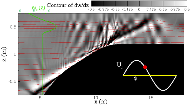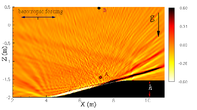
Bottom panel shows vertical x-z slice of the density field (after subtracting 1000 kg m −3) at 4 different times (phases) in a tidal cycle. Top panel shows spanwise-averaged streamwise velocities, u(z, t) m/s and density profiles, ρ(z, t, x = 0) at corresponding phases. Background linear density (dashed blue line) profile is also shown. Note that u, x are horizontal while z is vertical. Parts (a) and (e) correspond to maximum downward boundary flow, parts (b) and (f) correspond to flow reversal from down to up, parts (c) and (g) correspond to peak up-slope velocity and, finally, parts (d) and (e) correspond to flow reversal from up to down. The four different times are indicated by the four red color circles in Figure 4a that follows. Here, arrows are pointing the ow structures.	Preliminary results show an upward wave beam incident on realistic upper ocean stratification (buoyancy frequency profile is the green curve on the left). The phase of the barotropic tidal currents (white sine curve) is shown by the red dot. This figure is taken from ongoing work performed by Gayen and Sarkar.